Transformer系列：2. Attention机制，MHA，MQA和GQA

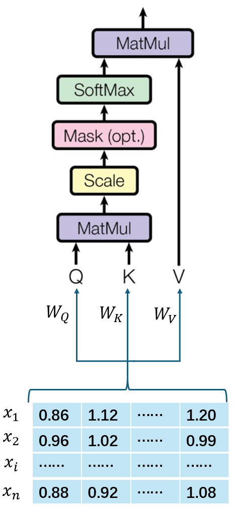
Scaled Dot-Product Attention

只使用一个注意力头计算权重。

假设有输入序列\(X=(x_1, x_2,..., x_n)\)，对于每个词\(x_i\)，计算其与所有其他词的相关性，并赋予不同的权重，最后对这些信息加权求和，得到新的表示。 \[ Attention(Q, K, V)=softmax(\frac{QK^{T}}{\sqrt{d_k}})V \]

分为以下几个步骤：

计算Query, Key, Value矩阵：每个输入token被映射为三个不同的向量：
- Q：当前需要关注的内容，例如在机器翻译中，查询可能是目标语言句子中的一个token；
- K：与查询进行匹配的内容，例如源语言句子中的token；
- V：最终要提取的信息，通常与键对应。
转换矩阵： \[ Q=XW_Q, K=XW_K, V=XW_V \] 其中，\(W_Q, W_K, W_V\)是可学习的参数矩阵。

输入：维度\(d_k\)的queries和keys；输出：维度为\(d_v\)的values
查询矩阵Q的维度：[\(n_q, d_k\)]，\(n_q\)为queries的数量；\(d_k\)是每个query的维度

键矩阵K的维度：[\(n_k, d_k\)]，\(n_q\)为keys的数量；\(d_k\)是每个key的维度

值矩阵V的维度：[\(n_k, d_v\)]，\(n_k\)为queries的数量；\(d_k\)是每个query的维度
1. Q和K的维度必须一致：V和Q/K的维度可以不一致；
2. K和V的长度必须一致：K和V本质上对应同一个sequence在不同空间的表达。
Attention得到的output：[\(n_q, d_v\)]，维度与V一致，长度与K一致。
计算点积：得到注意力分数矩阵 \[ scores=QK^{T} \]
缩放：将点积除以\(\sqrt{d_k}\)，其中：\(\sqrt{d_k}\)是Key向量的维度，\(\sqrt{d_k}\)是缩放因子，避免数值过大导致梯度消失。

为什么要使用缩放因子\(\sqrt{d_k}\)？ 归一化

假设\(Q, K\)里的元素均值为0，方差为1，那么：\(A=QK^{T}\)中元素均值为0，方差为\(d\)。当d变得很大时，\(A\)中的元素方差也变得很大，导致\(softmax(A)\)的分布也趋于陡峭（分布的方差大，分布集中在绝对值大的区域）。

\(A\)中每一个元素乘上\(\frac{1}{\sqrt{d_k}}\)后，方差又回到1，使得：\(softmax(A)\)的分布陡峭程度与\(d\)解耦，从而使得训练过程中，梯度值保持稳定。
softmax归一化：对缩放后的点积结果，应用softmax函数，得到注意力权重矩阵A： \[ A=softmax(\frac{QK^{T}}{\sqrt{d_k}}) \]
加权求和：将注意力权重矩阵\(A\)与值矩阵\(V\)相乘，得到加权求和的结果。

单头注意力机制代码实现：

import torch
import torch.nn as nn
import torch.nn.functional as F

class SingleHeadAttention(nn.Module):
    def __init__(self, embed_dim):
        """
        单头注意力机制的初始化。
        :param embed_dim: 嵌入维度，Query、Key 和 Value 的维度
        """
        super(SingleHeadAttention, self).__init__()
        self.embed_dim = embed_dim

        # 定义线性层，将输入映射到 Query、Key 和 Value
        self.query_linear = nn.Linear(embed_dim, embed_dim)
        self.key_linear = nn.Linear(embed_dim, embed_dim)
        self.value_linear = nn.Linear(embed_dim, embed_dim)

        # 缩放因子，用于防止点积结果过大
        self.scale = torch.sqrt(torch.FloatTensor($embed_dim]))

    def forward(self, query, key, value):
        """
        单头注意力的前向传播。
        :param query: 查询张量，形状为 $batch_size, seq_len_q, embed_dim]
        :param key: 键张量，形状为 $batch_size, seq_len_k, embed_dim]
        :param value: 值张量，形状为 $batch_size, seq_len_k, embed_dim]
        :return: 输出张量，形状为 $batch_size, seq_len_q, embed_dim]
        """
        # 将输入映射到 Query、Key 和 Value
        Q = self.query_linear(query)
        K = self.key_linear(key)
        V = self.value_linear(value)

        # 计算点积注意力分数
        attention_scores = torch.matmul(Q, K.transpose(-2, -1)) / self.scale

        # 应用 Softmax 函数，得到注意力权重
        attention_weights = F.softmax(attention_scores, dim=-1)

        # 加权求和，得到最终输出
        output = torch.matmul(attention_weights, V)

        return output, attention_weights

# 示例输入
# 假设我们有以下输入张量：
# - query: $batch_size, seq_len_q, embed_dim]
# - key: $batch_size, seq_len_k, embed_dim]
# - value: $batch_size, seq_len_k, embed_dim]
batch_size = 2
seq_len_q = 3# query的序列长度
seq_len_k = 4#k,v的序列长度，注意这里K、V是成对存在的
embed_dim = 6# 假设embedding的维度为6

# 随机生成输入数据
query = torch.randn(batch_size, seq_len_q, embed_dim)
key = torch.randn(batch_size, seq_len_k, embed_dim)
value = torch.randn(batch_size, seq_len_k, embed_dim)

# 初始化单头注意力模块
attention = SingleHeadAttention(embed_dim)

# 前向传播
output, attention_weights = attention(query, key, value)

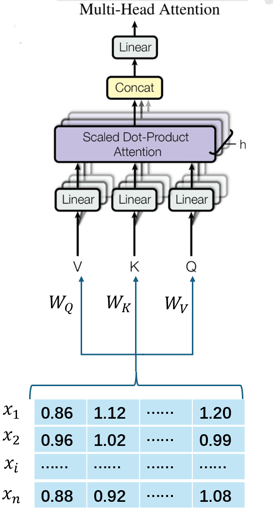
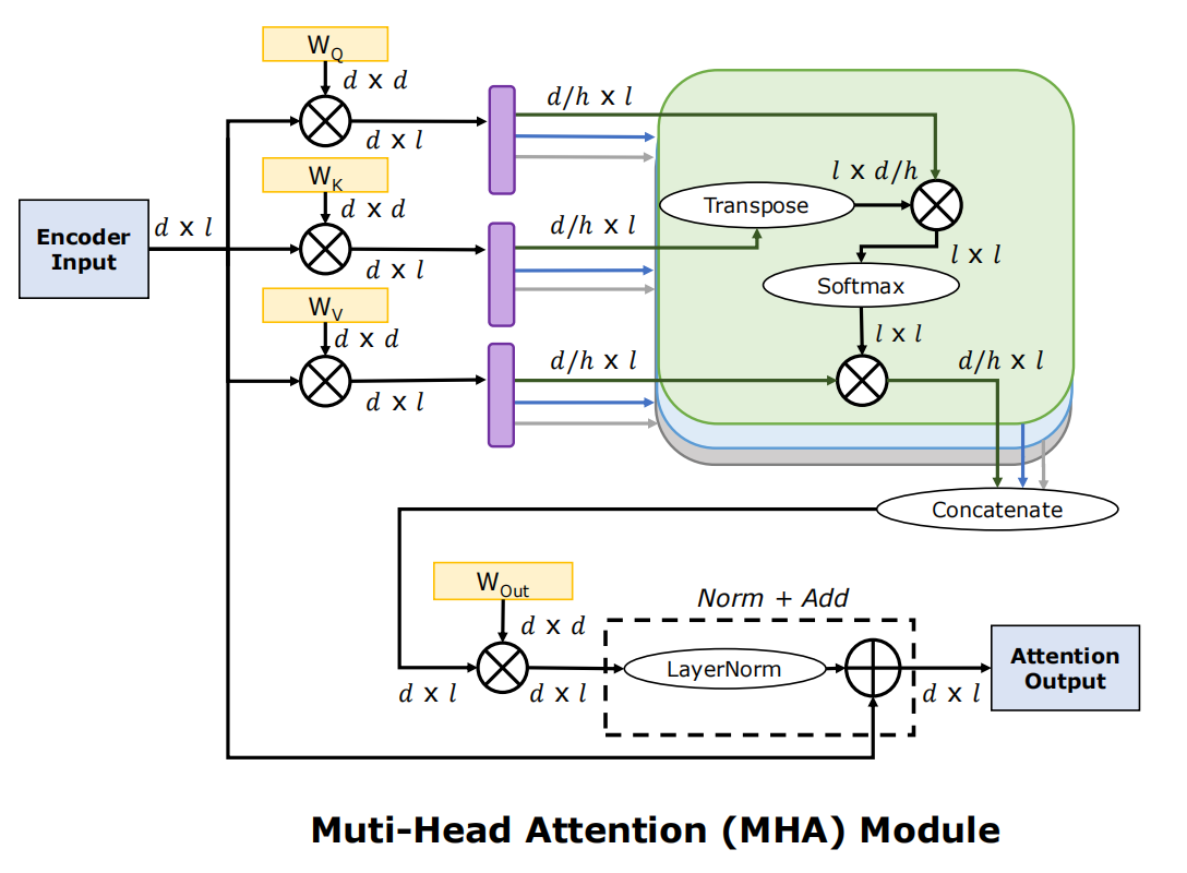
MHA

单头注意力中，模型只能通过一个注意力头来捕捉输入数据中的特征，这限制了模型对复杂关系的建模能力。而多头注意力（Multi-Head Attention）是Transformer架构的核心组件，它的核心思想是：将输入数据分解为多个子空间，每个子空间通过一个独立的注意力“头”（heads）进行处理，最后将所有heads的输出合并，从而能够捕捉到输入数据中不同子空间的特征；同时其复杂度并无增加。

步骤如下：

计算Query，Key，Value矩阵： \[ Q=XW_Q, K=XW_K, V=XW_V \]
分割多个heads：假设有\(h\)个heads，每个head的维度为\(d_k\)，则有： \[ d_k=\frac{d_{dim}}{h} \] 其中，\(d_{dim}\)是模型的嵌入维度。

分割后的Q，K，V如下： \[ Q_i=split(Q, i) \\ K_i=split(K, i) \\ V_i=split(V, i) \] 其中，\(i\)表示第\(i\)个头。
计算每个head的注意力：
1. 计算点积注意力分数： \[ A_i=Q_i\times K_i^{T} \]
2. 缩放： \[ S_i=\frac{A_i}{\sqrt{d_k}} \]
3. SoftMax： \[ W_i=softmax(S_i) \]
4. 加权求和： \[ O_i=W_i\times V_i \]
合并所有head的输出： \[ O=concat(O_1,O_2,...,O_h)W^{O} \]

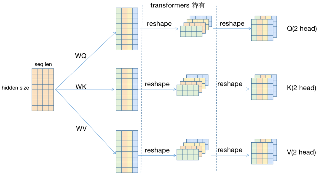
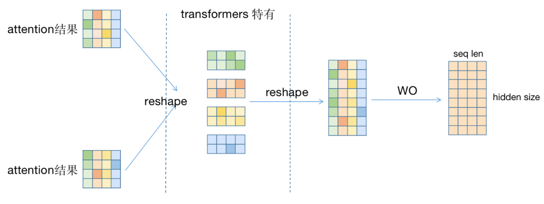
用一些示意图辅助理解：

假设输入序列的seq_len=4，hidden_size=8，使用2头注意力。弱化batch_size（假设为1）.

\(Q=XW_Q\)：\([s, h]\times [h, h]]\rightarrow [s, h]\)
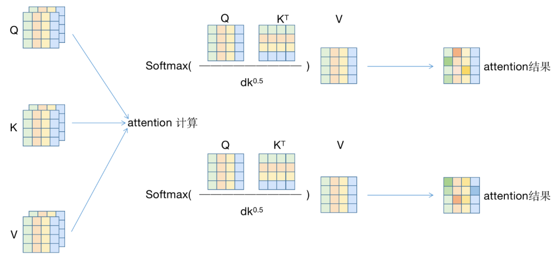
每个head：对于每个\(Q_i, K_i, V_i\)，分别计算attention，最后得到一个[2, 4, 4]的矩阵，即\([h, s, d_i]\). （引入head，切分hidden_size，设每个head的hidden_size为\(d_i\)）

\(QK^T=[h, s, d_i]\times [h, d_i, s]\rightarrow [h, s, s]\)
重新拼接为[8,4]的矩阵，即\([s, d]\)；再经过\(W_O\)，得到\(O\)矩阵，即输出。

MHA代码实现：

import torch
import torch.nn as nn
import torch.nn.functional as F

class MultiHeadAttention(nn.Module):
    def __init__(self, embed_dim, num_heads):
        """
        多头注意力机制的初始化。
        :param embed_dim: 嵌入维度
        :param num_heads: 头的数量
        """
        super(MultiHeadAttention, self).__init__()
        self.embed_dim = embed_dim
        self.num_heads = num_heads
        self.head_dim = embed_dim // num_heads

        assert self.head_dim * num_heads == embed_dim, "Embed size needs to be divisible by heads"

        # 定义线性层，将输入映射到 Query、Key 和 Value
        self.query_linear = nn.Linear(embed_dim, embed_dim)
        self.key_linear = nn.Linear(embed_dim, embed_dim)
        self.value_linear = nn.Linear(embed_dim, embed_dim)

        # 定义输出的线性层
        self.out = nn.Linear(embed_dim, embed_dim)

        # 缩放因子
        self.scale = torch.sqrt(torch.FloatTensor([self.head_dim]))

    def forward(self, query, key, value):
        """
        多头注意力的前向传播。
        :param query: 查询张量，形状为 [batch_size, seq_len_q, embed_dim]
        :param key: 键张量，形状为 [batch_size, seq_len_k, embed_dim]
        :param value: 值张量，形状为 [batch_size, seq_len_k, embed_dim]
        :return: 输出张量，形状为 [batch_size, seq_len_q, embed_dim]
        """
        batch_size = query.shape[0]

        # 将输入映射到 Query、Key 和 Value
        Q = self.query_linear(query)  # [batch_size, seq_len_q, embed_dim]
        K = self.key_linear(key)      # [batch_size, seq_len_k, embed_dim]
        V = self.value_linear(value)  # [batch_size, seq_len_k, embed_dim]

        # 分割成多个头
        Q = Q.view(batch_size, -1, self.num_heads, self.head_dim).transpose(1, 2)  # [batch_size, num_heads, seq_len_q, head_dim]
        K = K.view(batch_size, -1, self.num_heads, self.head_dim).transpose(1, 2)  # [batch_size, num_heads, seq_len_k, head_dim]
        V = V.view(batch_size, -1, self.num_heads, self.head_dim).transpose(1, 2)  # [batch_size, num_heads, seq_len_k, head_dim]

        # 计算点积注意力分数
        attention_scores = torch.matmul(Q, K.transpose(-2, -1)) / self.scale  # [batch_size, num_heads, seq_len_q, seq_len_k]

        # 应用 Softmax 函数，得到注意力权重
        attention_weights = F.softmax(attention_scores, dim=-1)  # [batch_size, num_heads, seq_len_q, seq_len_k]

        # 加权求和，得到每个头的输出
        output = torch.matmul(attention_weights, V)  # [batch_size, num_heads, seq_len_q, head_dim]

        # 合并所有头的输出
        output = output.transpose(1, 2).contiguous().view(batch_size, -1, self.embed_dim)  # [batch_size, seq_len_q, embed_dim]

        # 通过输出的线性层
        output = self.out(output)  # [batch_size, seq_len_q, embed_dim]

        return output, attention_weights

# 示例输入
batch_size = 2
seq_len_q = 3
seq_len_k = 4
embed_dim = 16
num_heads = 4

# 随机生成输入数据
query = torch.randn(batch_size, seq_len_q, embed_dim)
key = torch.randn(batch_size, seq_len_k, embed_dim)
value = torch.randn(batch_size, seq_len_k, embed_dim)

# 初始化多头注意力模块
attention = MultiHeadAttention(embed_dim, num_heads)

# 前向传播
output, attention_weights = attention(query, key, value)

KV Cache

大模型在decode阶段采用自回归的方式。即：最新的token输出依赖于先前生成或者预先填入的Token。

假如我们输入“窗前明月光下一句是”：decode过程如下：

step0: 输入=[BOS]窗前明月光下一句是；输出=疑
step1: 输入=[BOS]窗前明月光下一句是疑；输出=是
step2: 输入=[BOS]窗前明月光下一句是疑是；输出=地
step3: 输入=[BOS]窗前明月光下一句是疑是地；输出=上
step4: 输入=[BOS]窗前明月光下一句是疑是地上；输出=霜
step5: 输入=[BOS]窗前明月光下一句是疑是地上霜；输出=[EOS]

在生成“疑”字时，用的是输入序列中“是”字的最后一层hidden state，再通过最后的分类头预测。可以注意到：下一个step的输入包含了上一个step的内容，而且只在最后面多一个token；因此下一个step的计算也包含了上一个step的计算。

由于decoder是casual的（一个token的attention只依赖于之前的token，得益于mask attention）。因此在自回归生成的过程中，每一步会重复计算之前所有tokens的attention，可简化为：只计算新token的attention。

如下图：空的方块代表可以以前的steps中重用的计算部分：

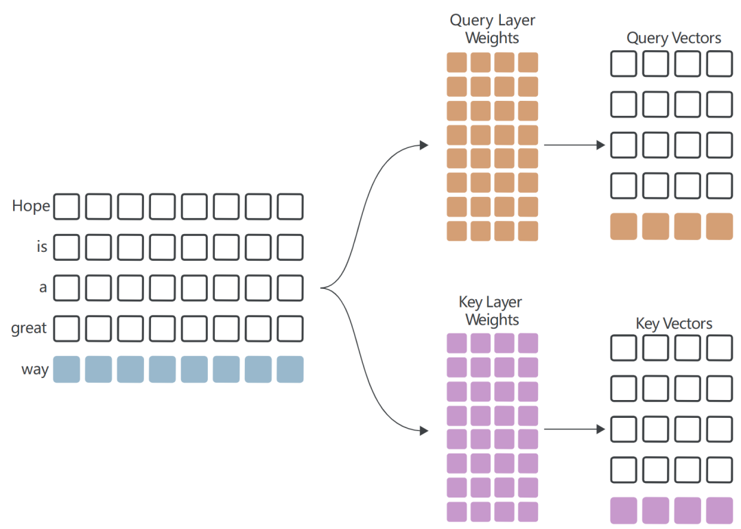
Key Cache

维护一个密钥缓存，存储：在每次迭代中计算的键向量。当前step的流程如下：

只计算一个Query向量和一个Key向量：
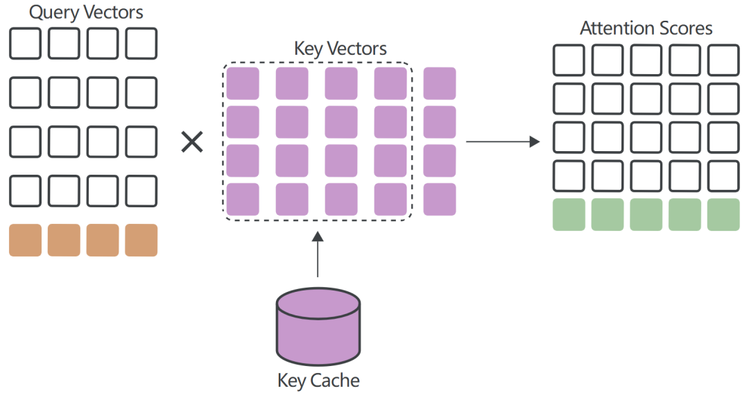
从Key Cache中提取先前steps计算的Key Vectors，计算Attention Score的最后一行，即新的Query Vector与所有Key Vectors的点积：

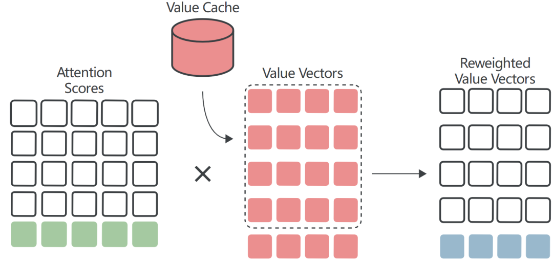
Value Cache

与Key Vector类似，每个step只需要计算最新的Value Vector；其他Value Vectors可以从Value Cache中提取并重复使用：

MQA

KV Cache虽然可以解决kv重复计算的问题，但面对长上下文时，显存占用量巨大。

以llama3-8B模型为例：模型序列长度\(L=8192\)(8K)；Transformer层数\(N=32\)，注意力头数\(H=32\)，每个注意力头的维度\(D=128\)，batch按照1算，数据类型为BF16（2个字节），需要的缓存为： \[ token_{kv}=2\times 1\times 32\times 8192\times 128\times 32\times 2=4294967296 \] 即4GB。

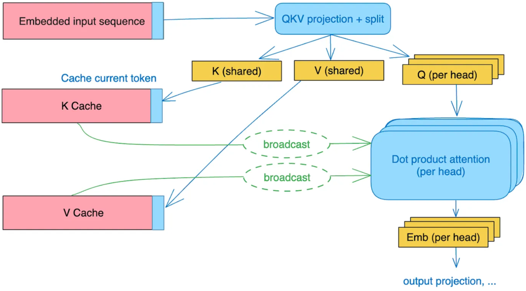
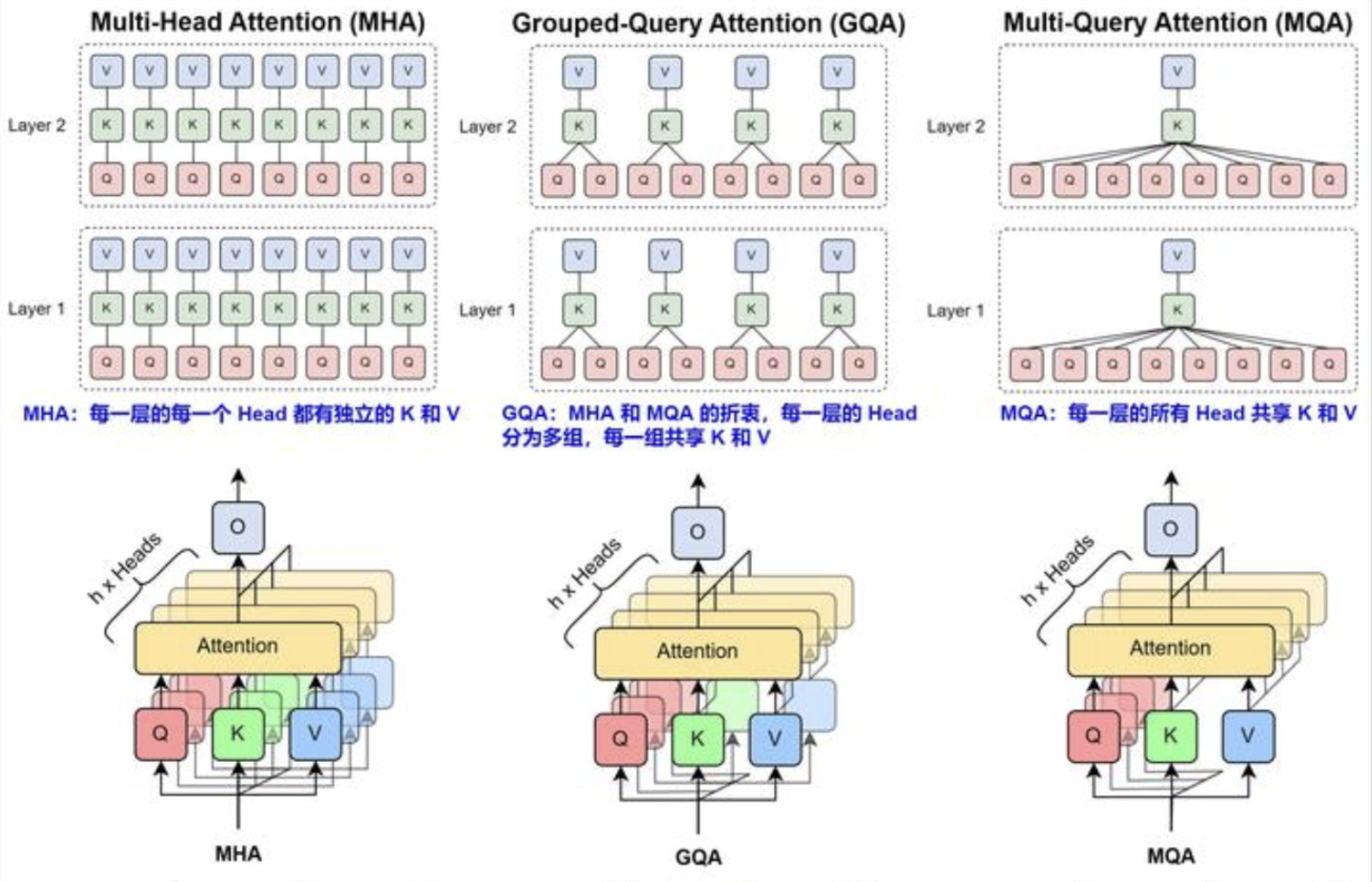
MQA的核心思想是：所有注意力头共享一份Key和Value矩阵，仅保留Query的多头性质。即：Key和Value的计算是唯一的，而Query则根据不同的头进行独立转换。

在下图中：

当 batch size=1 时，图中红色、绿色、蓝色虚线圈处的乘法全部为矩阵乘向量，是Memory Bound，算术强度不到 1。

当 batch size>1 时（比如 Continuous Batching）：

红色和蓝色部分：线性层计算是权重乘以激活，不同请求之间可以共享权重，因此是矩阵乘矩阵，并且 Batch Size 越大，算术强度越大，越趋近于计算密集型（FFN 层也类似）；

绿色部分：注意力计算是激活乘以激活。因为不同的请求之间没有任何相关性，即使 Batching，此处也是 Batched 矩阵乘向量，并且因为序列长度可能不同，这里不同请求的矩阵乘向量是不规则的。即，这里算术强度始终不到 1，是Memory Bound。

因此绿色部分较难优化，输入序列越长，瓶颈越大。

与MHA对比：

MHA：输入分别经过\(W_Q, W_K, W_V\)的变换，切成\(n\)份（n为头数），维度从\(d_{model}\)降到\(d_{head}\)，分别进行attention计算再拼接；

MQA：只对\(Q\)切分，而\(K, V\)直接在线形变换时将维度降至\(d_{head}\)（而不是切分变小）

假设输入的维度为：\([b, s, d]\)，其中\(b\)为batch size，\(s\)为sequence length，\(d\)为hidden size。

线性变换：得到的\(Q\)为\([b, s, d]\)；\(K, V\)为\([b, s, d_head]\).

多头切分：

将\(Q\)按head切分：

1	Q = Q.view(batch_size, -1, self.num_heads, self.head_dim).transpose(1, 2)

拓展\(K, V\)以匹配\(Q\)的维度：

1 2	K = K.unsqueeze(1).expand(-1, self.num_heads, -1, -1) V = V.unsqueeze(1).expand(-1, self.num_heads, -1, -1)

注意力计算：计算\(Q, V\)之间的点积： \[ scores=\frac{Q_{split}K_{split}^T}{\sqrt{d_{head}}} \] 应用softmax获取注意力权重： \[ W=softmax(scores) \] 使用注意力权重，对Value加权求和： \[ context=WV_{split} \]

多头合并：使用矩阵乘法 matmul广播，使得每个头都乘以这同一个张量，以此来实现KV参数共享。

1
2
3

output = torch.matmul(attn, V)  
# (batch_size, num_heads, seq_len, head_dim)
output = output.transpose(1, 2).contiguous().view(batch_size, -1, self.d_model) # (batch_size, seq_len, d_model)

数学公式：

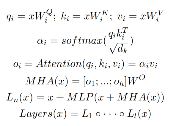
MQA代码实现：

import torch
import torch.nn as nn
import torch.nn.functional as F

class MultiQueryAttention(nn.Module):
    def __init__(self, d_model, num_heads):
        super(MultiQueryAttention, self).__init__()
        self.num_heads = num_heads
        self.d_model = d_model
        self.head_dim = d_model // num_heads

        assert (
            self.head_dim * num_heads == d_model
        ), "d_model must be divisible by num_heads"

        self.query_linear = nn.Linear(d_model, d_model)
        self.key_linear = nn.Linear(d_model, self.head_dim)
        self.value_linear = nn.Linear(d_model, self.head_dim)
        self.out_linear = nn.Linear(d_model, d_model)

    def forward(self, queries, keys, values, mask=None):
        batch_size = queries.size(0)

        # 线性变换
        Q = self.query_linear(queries)  # (batch_size, seq_len, d_model)
        K = self.key_linear(keys)       # (batch_size, seq_len, head_dim)
        V = self.value_linear(values)   # (batch_size, seq_len, head_dim)

        # 分割为多个头
        Q = Q.view(batch_size, -1, self.num_heads, self.head_dim).transpose(1, 2)  # (batch_size, num_heads, seq_len, head_dim)
        K = K.unsqueeze(1).expand(-1, self.num_heads, -1, -1)                      # (batch_size, num_heads, seq_len, head_dim)
        V = V.unsqueeze(1).expand(-1, self.num_heads, -1, -1)                      # (batch_size, num_heads, seq_len, head_dim)

        # 计算注意力得分
        scores = torch.matmul(Q, K.transpose(-2, -1)) / torch.sqrt(torch.tensor(self.head_dim, dtype=torch.float32))
        if mask isnotNone:
            scores = scores.masked_fill(mask == 0, -1e9)
        attn = F.softmax(scores, dim=-1)
        # 计算注意力输出
        output = torch.matmul(attn, V)  # (batch_size, num_heads, seq_len, head_dim)
    
        output = output.transpose(1, 2).contiguous().view(batch_size, -1, self.d_model)  # (batch_size, seq_len, d_model)

        return self.out_linear(output)

batch_size = 1
seq_len = 3
d_model = 4
num_heads = 2

# 随机生成输入张量
queries = torch.rand(batch_size, seq_len, d_model)
keys = torch.rand(batch_size, seq_len, d_model)
values = torch.rand(batch_size, seq_len, d_model)

# 初始化 MQA 模型
mqa = MultiQueryAttention(d_model, num_heads)

mask = torch.tril(torch.ones(seq_len, seq_len)).unsqueeze(0).unsqueeze(0)  # (1, 1, seq_len, seq_len)
print('mask:',mask)
# 前向传播
output = mqa(queries, keys, values,mask)

print("输出张量：")
print(output)

内存

MQA所需要缓存的KV值，从所有头减为一个头，KV Cache减少为之前的\(\frac{1}{h}\)。

性能测试如下：

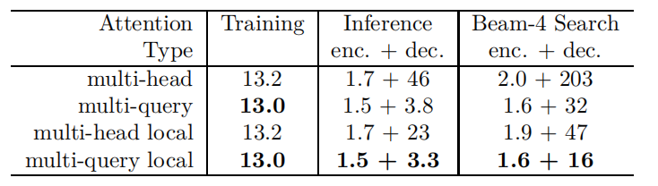
训练速度基本不变；
推理时间和beam-search时间大幅缩短；
推理过程中：Encoder推理速度基本不变；Decoder推理大幅加速。

MQA不改变计算量，但大幅降低了显存使用（降低KV Cache）：

降低KV Cache的空间占用率；节省的显存空间可用于增加批次大小、提升吞吐量；
头数量的减少，导致从显存中读取的数据量减少，减少了计算单元的等待时间，从内存密集型趋近于计算密集型。

表征能力

共享K，V可能导致模型捕捉上下文的能力下降，限制模型的表征能力，导致任务效果相比MHA略有损失。

通信

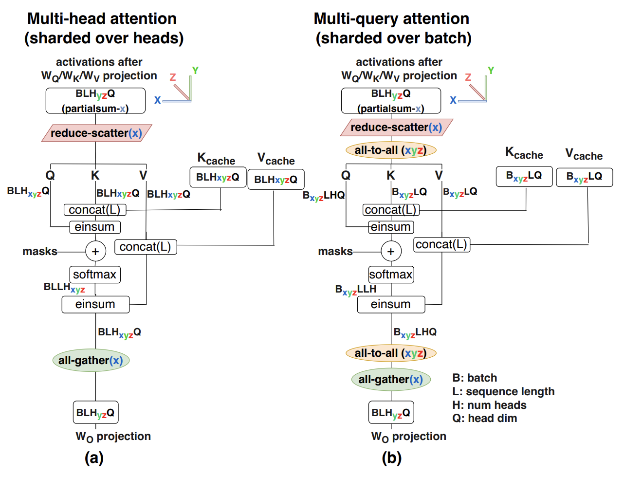
在多卡并行情况下，MQA减少了访存，但是增加了并行通信开销。由于K和V张量在所有头部之间共享，每个GPU上都需要有自己的备份。与下图(a)中MHA并行策略相比，MQA需要使用all-to-all对进行输入输出激活张量resharding，从而产生额外的通信成本。具体如下图(b)所示。另外，因为每个卡上都有备份，这可能会导致MQA的内存成本节省将会丧失。

GQA

MHA和MQA的折中方案：采用分组机制，让多个 Query 共享少量的 Key 和 Value，减少自注意力计算的复杂度，同时保持 Transformer 的表达能力。

Query多头计算：Query依然是每个头独立计算。假设有\(h\)个注意力头，计算方式如下： \[ Q_i=XW_Q^i, i=1,2,...,h \] 其中：\(W_Q^i\)是第\(i\)个头的Query投影矩阵；计算出的\(Q_i\)形状为\([b, s, d_{head}]\).（\(d_head=\frac{d}{h}\)）
共享分组：Key和Value计算。将Key和Value分成\(g\)组，其中\(g<h\)，即： \[ K_j=XW_K^j, V_j=XW_V^j, j=1,2,...,g \] 计算出的\(K_j, V_j\)形状为\([b, s, d_g]\)（\(d_g=\frac{d}{g}\)）
计算注意力分数： \[ A_i=softmax(\frac{Q_iK_j^T}{\sqrt{d_g}}) \] 其中：\(Q_i\)来自每个Query头；\(K_j\)来自共享的Key组。计算得到的\(A_i\)形状为\([b, s, s]\).
计算加权Value： \[ Z_i=A_iV_j \]

其中：\(V_j\)是共享的Value组。计算得到的\(Z_i\)形状为\([b, s, d_{head}]\)

输出计算：拼接所有注意力头计算的结果\(Z_i\)会被拼接： \[ Z=[Z_1, Z_2, ..., Z_h]W_O \] 其中，\(W_O\)是输出投影矩阵，最终得到形状为\([b, s, d]\)的输出。

GQA代码实现：

import torch
import torch.nn as nn

class GQA(nn.Module):
    def __init__(self, d_model, num_heads, num_groups):
        super(GQA, self).__init__()
        assert num_heads % num_groups == 0, "Heads should be evenly divisible by groups"
        self.num_heads = num_heads
        self.num_groups = num_groups
        self.d_model = d_model
        self.d_head = d_model // num_heads
        self.d_group = d_model // num_groups  # Key-Value 分组维度

        # Query 仍然是独立的
        self.W_q = nn.Linear(d_model, d_model, bias=False)
        # Key 和 Value 共享
        self.W_k = nn.Linear(d_model, d_model // num_groups * num_heads, bias=False)
        self.W_v = nn.Linear(d_model, d_model // num_groups * num_heads, bias=False)
        self.W_o = nn.Linear(d_model, d_model, bias=False)
    
    def forward(self, x):
        batch_size, seq_len, _ = x.shape

        # 计算 Query, Key, Value
        Q = self.W_q(x).view(batch_size, seq_len, self.num_heads, self.d_head)
        K = self.W_k(x).view(batch_size, seq_len, self.num_groups, self.d_group)
        V = self.W_v(x).view(batch_size, seq_len, self.num_groups, self.d_group)

        # 计算注意力分数
        attention_scores = torch.einsum("bqhd,bkgd->bhqk", Q, K) / (self.d_group ** 0.5)
        attention_weights = torch.softmax(attention_scores, dim=-1)

        # 计算注意力加权值
        Z = torch.einsum("bhqk,bkgd->bqhd", attention_weights, V)

        # 重新 reshape 并输出
        Z = Z.reshape(batch_size, seq_len, self.d_model)
        return self.W_o(Z)

MHA，MLA，MQA对比：

在MHA下，对于所有输入批次和序列中的每个token，KV Cache的总大小为： \[ 2\times b\times l\times h\times d\times n \] 其中，\(b\)为batch size，\(l\)为总序列长度（输入+输出序列），\(h\)为注意力头数量，\(d\)为每个head的维度，\(n\)为层数。

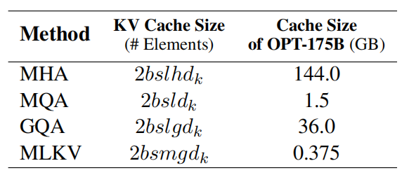
上图中，\(g\)为KV头的组数。当\(g=h\)时是MLA；当\(g=1\)时是MQA；当\(1<g<h\)时，只将KV Cache压缩到\(\frac{g}{h}\)。

GQA和MQA的性能收益主要来源于KV Cache的减少，支持放入更多tokens；但GQA和MQA的性能容易受到并行策略的影响。

GQA和MQA的瓶颈主要在于加载 KV。如果GQA kernel在Q head维度上做并行（一个Q head对应一个block），则会导致共享一个KV head的block被调度在不同的SM上，每个SM 都会对同一份KV head 做重复加载。则内存减少的收益会大大降低。因此需要减少Q head的并行度。

在llama2/3-70B中，GQA中\(g=8\)，其他用了GQA的同体量模型基本上也保持了这个设置，这是出于对推理效率的考虑。70B体量的模型，如果不进行极端的量化，不可能部署到单卡（A100/H100 80G）上；一般情况下一台机可以装8张卡，而Attention的每个Head实际上是独立运算然后拼接起来的，因此，正好可以每张卡负责计算一组K、V对应的Attention Head。这样可以在尽可能保证K、V多样性的同时最大程度上减少卡间通信。